This is the second blog on getting started with Statistics for Oracle Data Science projects.
- The first blog post in the series looked at the DBMS_STAT_FUNCS PL/SQL package, what it can be used for and I give some sample code on how to use it in your data science projects. I also give some sample code that I typically run to gather some additional stats.
- The second blog post will look at some of the other statistical functions that exist in SQL that you will/may use regularly in your data science projects.
- The third blog post will provide a summary of the other statistical functions that exist in the database.
In this blog post I will look at 3 more useful statistical functions that are available in the Oracle database. Remember these come are standard with the database. The first function I will look at is the WIDTH_BUCKET function. This can be used to create some histograms of the data. A common task in analytics projects is to produce some cross tabs of the data. Oracle has the STATS_CROSSTAB. The last function I will look the different ways you an sample the data.
Histograms using WIDTH_BUCKET
When exploring your data it is useful to group values together into a number of buckets. Typically you might want to define the width of each bucket yourself before passing the data into your data mining tools, but before you can decide what these are you need to do some exploring using a variety of widths. A good way to do this is to use the WIDTH_BUCKET function. This takes the following inputs:
Expression: This is the expression or attribute on which the you want to build the histogram.
Min Value: This is the lower or starting value of the first bucket
Max Value: This is the last or highest value for the last bucket
Num Buckets: This is the number of buckets you want created.
Typically the Min Value and the Max Value can be calculated using the MIN and MAX functions. As a starting point you generally would select 10 for the number of buckets. This is the number you will change, downwards as well as upwards, to if a particular pattern exists in the attribute.
Using the example scenario that I used in the first blog post, let us start by calculating the MIN and MAX for the AGE attribute.
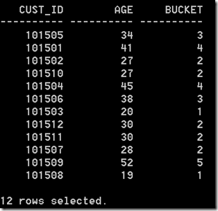
Lets say that we wanted to create 10 buckets. This would create a bucket width of 7.3 for each bucket, giving us the following.
Bucket 1 : 17-24.3
Bucket 2: 24.3-31.6
Bucket 3: 31.6-38.8
Bucket 4: 38.8-46.1
Bucket 5: 46.1-53.4
Bucket 6: 53.4-60.7
Bucket 7: 60.7-68
Bucket 8: 68-75.3
Bucket 9: 75.3-82.6
Bucket 10: 82.6-90
These are the buckets that the WIDTH_BUCKET function gives us in the following:
SELECT cust_id,
age,
width_bucket(age,
(SELECT min(age) from mining_data_build_v),
(select max(age)+1 from mining_data_build_v),
10) bucket
from mining_data_build_v
where rownum <=12
group by cust_id, age
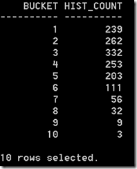
An additional level of detail that is needed to allow us to plot the histograms for AGE, we need to aggregate up for all the records by bucket.
select intvl, count(*) freq
from (select width_bucket(salary,
(select min(salary) from employees),
(select max(salary)+1 from employees), 10) intvl
from HR.employees)
group by intvl
order by intvl;
We can take this code and embed it into the GATHER_DATA_STATS procedure that I gave in my Part 1 blog post.
Cross Tabs using STATS_CROSSTAB
Typically cross tabulation (or crosstabs for short) is a statistical process that summarises categorical data to create a contingency table. They provide a basic picture of the interrelation between two variables and can help find interactions between them.
Because Crosstabs creates a row for each value in one variable and a column for each value in the other, the procedure is not suitable for continuous variables that assume many values.
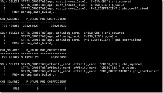
In Oracle we can perform crosstabs using one of their reporting tools. But if you don’t have one of these we will need to use the in-database function STATS_CROSSTAB. This function takes three parameters, the first two of these are the attributes you want to compare and the third is what test we want to perform. The tests available include:
- CHISQ_OBS: Observed value of chi-squared
- CHISQ_SIG: Significance of observed chi-squared
- CHISQ_DF: Degree of freedom for chi-squared
- PHI_COEFFICIENT: Phi coefficient
- CRAMERS_V: Cramer’s V statistic
- CONT_COEFFICIENT: Contingency coefficient
- COHENS_K: Cohen’s kappa
CHISQ_SIG is the default.
Now let us look at some examples using our same data set.
Sampling Data
When our datasets are of relatively small size consisting of a few hundred thousand records we can explore the data is a relatively short period of time. But if your data sets are larger that that you may need to explore the data by taking a sample of it. What sampling does is that it takes a “random” selection of records from our data set up to the new number of records we have specified in the sample.
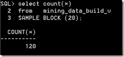
In Oracle the SAMPLE function takes a percentage figure. This is the percentage of the entire data set you want to have in the Sampled result.
There is also a variant called SAMPLE BLOCK and the figure given is the percentage of records to select from each block.
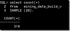
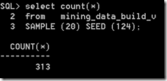
Each time you use the SAMPLE function Oracle will generate a random seed number that it will use as a Seed for the SAMPLE function. If you omit a Seed number (like in the above examples), you will get a different result set in each case and the result set will have a slightly different number of records. If you run the sample code above over and over again you will see that the number of records returned varies by a small amount.
If you would like to have the same Sample data set returned each time then you will need to specify a Seed value. The Seed much be an integer between 0 and 4294967295.
In this case because we have specified the Seed we get the same “random” records being returned with each execution.

No comments:
Post a Comment