This is a the second part of a five (5) part blog post on building and using Clustering in Oracle Data Miner. The following outlines the contents of each post in this series on Clustering.
- The first part we looked at what clustering features exist in ODM and how to setup the data that we will be using in the examples
- The second part will focus on how to building Clusters in ODM .
- The third post will focus on examining the clusters produced by ODM and how to use the Clusters to apply to new data using ODM.
- The fourth post will look at how you can build and evaluate a Clustering model using the ODM SQL and PL/SQL functions.
- The fifth and final post will look at how you can apply your Clustering model to new data using the ODM SQL and PL/SQL functions.
With Clustering we are trying to find hidden patterns in our data. Unlike classification we a not directing the algorithms on what areas/attributes to focus on.
In our scenario we want to look to see what distinct groupings or Segments that our Customer data naturally fit into. For each of these Segment Oracle Data Miner will tell us what attributes and the values of these attributes that determine if a customer belongs to one segment or another.
Step 1 - Define the Data Source
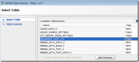
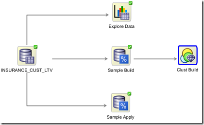
The first step involves us creating a Data Source Node for the table that we created and loaded in the previous blog post. We called this table INSURANCE_CUST_LTV.
To create the Data Source Node go to the Component Palette. Under the Data tab you will find the Data Source option. Click on this and then go to the workflow worksheet and click. The Data Source node will be created and the wizard to specify the name of the table/view will open. Select INSURANCE_CUST_LTV from the list.
Click on the Next and then the Finish button to take in all the attribute.
Our data is now read to use.
Step 2 – Explore the Data
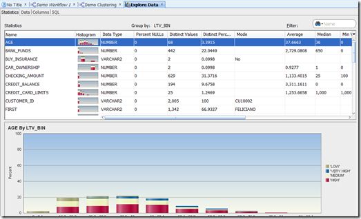
We can use the Explore Node to gather some statistics on the data and to produce some graphs.
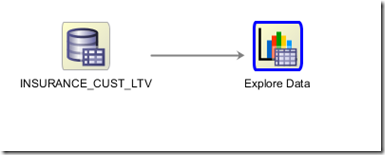
To create the Explore Node, go to the Component Palette and under the Data tab you will find the Explore Data node. Click on this and then click again on the workflow worksheet, near the Data node.
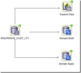
You need to connect the Data node to the Explore Data node. Move your mouse to the Data node. Right-click this node and select Connect from the drop down menu. Then more the mouse to the Explore Data node and click on it. You will now have an arrowed line joining these two nodes
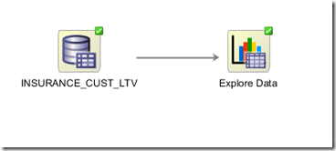
The next step we need to do is to right click on the Explore Data node and select Run from the drop down menu. ODM will go off to the database and gather various statistics and create a number of graphs based on the data in the table.
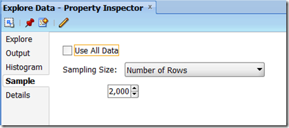
NB. If you click on the Explore Data node and then look in the Property Inspector you will see that ODM will take a sample of 2,000 records to produce the statistics and graphs. If you would like ODM to use all the records then you need to click the ‘Use All Data’ check box. Or you can change the sample size.
For your initial data investigation you might use the default of sampling 2,000 records before you increase the size of the sample.
In scenarios like this you may want to explore the data in more detail and to look at how the data is distributed in relation to certain attributes. In our data we have an attribute called LTV_BIN. In this attribute we have four values including, Very High, High, Medium and Low.
In our scenario, it might be more interesting to explore the data based on this attribute and it’s values. To do this we need to tell the Explore Data node to group the data analysis based on the values in this attribute.
Double-click the Explore Data node. In the Group By drop down select LTV_BIN. Click the OK button. You are now ready to run the Explore Data Node. To do this, right click on Explore Data node and select Run from the drop down list.
To view the statistics gathered and the graphs produced on the default sample of 2,000 records, right click the Explore Data node and select View Data from the drop down menu. You will get a new tab/window opening in SQL Developer with all the results.
This kind of data analysis only works with an attribute that has a low number of possible values.
Step 3 – Defining the data we will used to Build our Cluster models
We are going to divide the data in our CUST_INSURANCE_LTV into two data sets. The first data set will be used to build the Cluster models. The second data set will be used as part of the Apply node in my next blog post (part 3).
To divide the data we are going to use the Sample Node that can be found under the Transformation tab of the Component Palette.
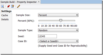
Create your first Sample Node. In the Settings tab of the Property Inspector set the sample size to 60% and in the Details tab rename the node to Sample Build.
Create a second Sample node and give it a sample size of 40%. Rename this node to Sample Apply.
Right click on each of these Sample nodes to run them and have them ready for the next step of building the Clustering models.
Step 4 – Creating the Clustering Build Node
When you have finished exploring the data you are now ready to move on to creating the Clustering models. As ODM has two clustering algorithms, ODM will default to creating two Clustering models.
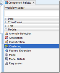
To create the Clustering models, go to the Component Palette. Under the Models tab, select Clustering.
Move the mouse to the workflow worksheet, near the Sample Build node and click the worksheet. The Clustering node will be created. Now we need to connect the data with the Clustering node. To do this right click on the Sample Build node and select Connect from the drop down list. Then move the mouse to the Clustering node and click. An arrowed line will be created connecting the two nodes.
At this point we can run the Clustering Build node or we can have a look at the setting for each algorithm.
Step 5 – The Clustering Algorithm settings
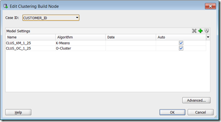
To setup the Cluster Build node you will need to double click on the node to open the properties window. The first thing that you need to do is to specify the Case ID (i.e. the primary key). In our example this is the CUSTOMER_ID.
Oracle Data Miner has two clustering algorithms. The first of these is the well know k-Means (it is an enhanced version of it) and the O-Cluster. To look at the settings for each algorithm, click on the model listed under Model Settings and then click on the Advanced button.
A new window will open that lists all the attributes for the in the data source. The CUSTOMER_ID is unchecked as we said that this was the CASE_ID.
Click on the Algorithm Settings tab to see the internal settings for the k-means algorithm. All of these settings have a default value. Oracle has worked out what the optimal setting are for you. The main setting that you might want to play with is the Number of Clusters to build. The default is 10, but you might want to play with numbers between 5 and 15 depending on the number of clusters or segments you want to see in your data.
To view the algorithm settings for O-Cluster click on this under the Model Setting. We have less internal settings to worry about here, but we again can determine how many clusters we want to produce.
For our scenario we are going to take the default settings.
Step 6 – Run/Generate the Clustering models
At this stage we have the data set-up, the Cluster Build node created and the algorithm setting all set to what we want.
Now we are ready to run the Cluster Build node.
To do this, right click on the Cluster Build node and click run. ODM will go create a job that will contain PL/SQL code that will generate a cluster model based on K-Means and a second cluster model based on O-Cluster. This job will be submitted to the database and when it is completed we will get the little green tick mark on the top right hand corner of the Cluster Build node.
In the next blog post we will look at how to examine what clusters were produced by ODM and how we can take one of these and apply them to new data.
No comments:
Post a Comment